Standalone version to add custom genome sets
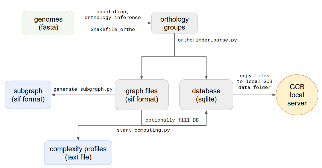
Standalone version should be used when the user wants to work with a custom set of genomes. Command-line scripts are provided to: calculate complexity profile, generate subgraphs, generate a database which can be imported to browser-based GUI application. Scheme of actions and scripts is shown below.
Requirements
- snakemake
- python3 with libraries:
- biopython
- gene-graph-lib
- ???
- OrthoFinder
- prokka
The best way to get ready for the analysis is to use conda. If you have no conda in your system, start with installing it: https://docs.conda.io/projects/conda/en/latest/user-guide/install/linux.html
Orthology group inference
Orthogroup inference is the first step in the standalone analysis. We recomend using our orthosnake pipeline to perfrom orthogroup inference, because GCB requires some special formating of the files. If you want to perform this step without orthosnake pipeline, you will find the specifications of the formats used HHEERREE.
Orthosnake pipeline
INPUT: Fasta-formated files with .fna extension, one file per genome. *OUTPUT: orthogroups file `Orthogroups.txt` in OrthoFinder format
Steps:
- Clone or download orthosnake GIT repository: https://github.com/paraslonic/orthosnake
- Put fasta-formated genome files in fna folder of the orthosnake folder.
- Rut snakemake with appropriate settings
Example:
If genome files have extension other than .fna please rename them, i.e. with following command: for i in fna/*.fasta; do mv $i fna/$(basename $i .fasta).fna; done
### Algorightm
- Fasta files headers are modified to be consistent with Prokka: * if header contains symbols other than alphanumericals and _ they are converted to _ * if header is longer than 20 symbols it is cropped to first 18 symbols and dots are added to the end (i.e. gi|15829254|ref|NC_002695.1 becomes gi|15829254|ref|NC..)
- Annotation with Prokka
- Amino acid fasta files are generated from genebank files; gene location and product information are listed in headers.
- Orthogroups are inferred with OrthoFinder.
Generating of the graph structure
Graph structure is stored in text file with sif format, and in database When orthogroups are inferred, the next step is parsing of Orthofinder outputs. To do this you should open source directory and type in terminal:
python3 orthofinder_parse.py -i [path to txt file with orthogroups] -o [path and name prefix for output files]
For example:
python3 orthofinder_parse.py -i ~/data/Mycoplasma/Results/Orthogroups.txt -o ~/data/outputs/Mycoplasma/graph
Output files:
graph.sif- all edges list of the genomes graphgraph.db- SQLite database with all parsed informationgraph_context.sif- number of unique contexts, computed for each node in the graphgraph_genes.sif- list of all genes (nodes) from all genomes, with coordinates and Prokka annotations
The main graph structure is stored in a text graph.sif file, where each one line describes one edge, with its source and target nodes, genome id and contig id, to which this edge belongs. This file is used to create a graph object, which is used in all graph processing procedures.
Complexity computing
The next step is the computing of genome complexity. To do this type in terminal:
python3 start_computing.py -i graph.sif -o [path to output folder] --reference [name of reference genome]
- Additional parameters:
–window - sliding window size (default 20)
–iterations - number of iterations in probabilistic method (default 500)
–genomes_list - path to file with a list of names which will be used to create a graph (default all strains from *.sif will be used)
–min_depth, –max_depth - minimum and maximum depth of generated paths in the graph (default from 0 to inf)
–save_db - path to the database, created by orthfinder_parse.py (default data will not be saved to db, only to txt). It’s necessary to use this parameter if you want to use this complexity profile in the stand-alone browser-based GCB application.
Output files for each contig in the reference genome:
all_bridges_contig_n.txt- this file contains information about the number of deviating paths between each pair of nodes in the reference genome
PODVAL
Then gene annotation with prokka tool of each genome is performed. Genbank files then converted to fasta formatted amino acid protein sequences with a custom python3 script. This script inserts special information about genes in fasta headers, namely: genome file name, numeric id, product name, contig, start, end (for example, >GCF_000007445|4|Threonine_synthase|NC_004431.1|4445|5731). Then these files are used to infer orthology groups with OrthoFinder tool. The resulting file with orthology groups (OG) contains information about each OG in the following format: <og id>: <gene1> <gene2> …
For example:
OG0008594: GCF_001618325|2406|Small_toxic_polypeptide_LdrD|NZ_CP015069.1|2607133|2607240 GCF_001663475|366|Small_toxic_polypeptide_LdrD|NZ_CP015159.1|380042|380149